Note
Go to the end to download the full example code.
Seismic Data Plotting#
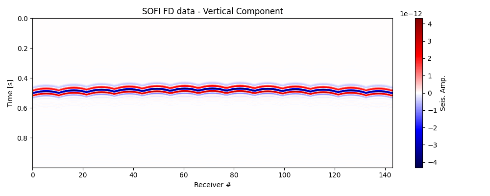
This example shows how to visualise seismic trace data as an image, which is particularly useful when handling a large number of traces.
import matplotlib.pyplot as plt
import numpy as np
import os
from fracspy.utils.sofiutils import read_seis
from fracspy.visualisation.traceviz import traceimage


plt.close("all")
np.random.seed(0)
Data Loading#
Load data previously modelled using SOFI3D finite difference package
# Directory containing input data
input_dir = '../data/pyfrac_SOFIModelling'

# Load receiver geometry - required to know number of receivers
recs_xzy = np.loadtxt(os.path.join(input_dir,'inputs',
                                   'griddedarray_xzy_20m.dat')).T
nr = recs_xzy.shape[1]

# Modelling parameters
dt = 1e-3  # SOFI3D Time sampling rate

# Load seismic data
expname = 'explosive_Homogeneous_griddedarray'
vz = read_seis(os.path.join(input_dir, 'outputs',
                            'su', f'{expname}_vy.txt'),
               nr=nr)
Traces as an Image Visualisation#
Where there are a relatively small number of traces (<40), wiggle plots can be particularly useful for identifying events.
fig, ax = traceimage(vz, dt=dt, climQ=99.99, figsize=(10, 4))
ax.set_title('SOFI FD data - Vertical Component')
plt.tight_layout()

Total running time of the script: (0 minutes 0.213 seconds)
