Detection Function Plotting

This example shows how to visualise detection functions (curves), e.g. when working with diffraction stacking detection.

import numpy as np
import matplotlib.pyplot as plt
from scipy.stats import norm
from fracspy.visualisation.plotting_support import detection_curves
from fracspy.detection.stacking import stalta

Create simple dataset

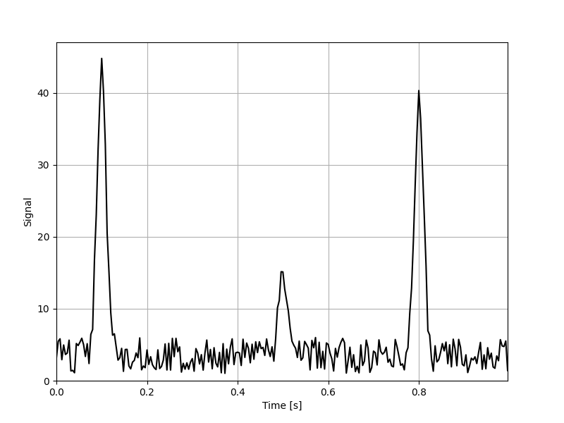
Here we generate a purely synthetic function which would look like a maximum stack function

# Parameters
dt = 0.004  # time step in seconds
duration = 1.0  # total duration of the signal in seconds
t = np.arange(0, duration, dt)  # time array

# Gaussian function parameters: mean, standard deviation, maximum
gaussian_params = [
    {"mean": 0.1, "std": 0.01, "height": 1},    # First peak
    {"mean": 0.5, "std": 0.01, "height": 0.3},  # Second peak
    {"mean": 0.8, "std": 0.01, "height": 0.9},  # Third peak
]

# Create the signal with constant level of 1
signal = np.zeros_like(t) + 1


# Add each Gaussian peak to the signal
for params in gaussian_params:
    gaussian = params["height"] * norm.pdf(t, params["mean"], params["std"])
    signal += gaussian

# Generate random background noise between 0 and 5
random_noise = np.random.uniform(0, 5, size=len(t))

# Add the random background noise to the signal
signal += random_noise

Plot the function

fig,axs = detection_curves(msf=signal,t=t,msflabel='Signal',figsize=(8, 6))

#%

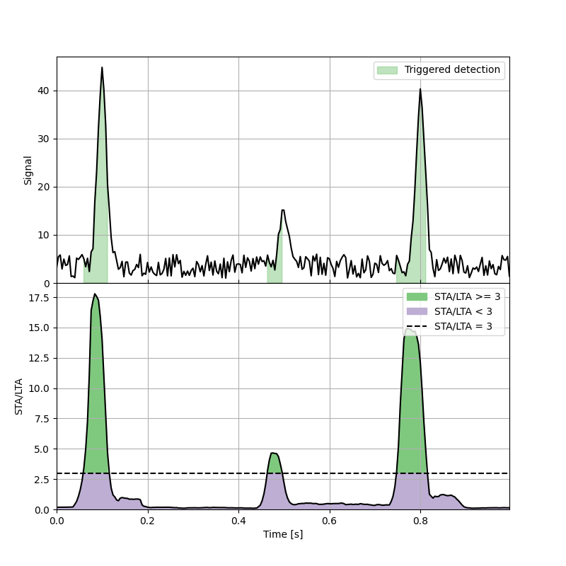
Get Short Term Average / Long Term Average (STA/LTA)

Set parameters

# Short time window
stw = 0.05

# Long time window
ltw = 5*stw

# Gap time window
gtw = 1

# Compute STA/LTA for the example signal
slf,_,_ = stalta(tdf=signal, dt=dt, stw=stw, ltw=ltw, gtw=gtw)

Plot both the signal and the STA/LTA

fig,axs = detection_curves(msf=signal,t=t,msflabel='Signal',slf=slf)