Event Volume Plotting

This example shows how to visualise microseismic event characteristics, i.e., semblance or imaging functions as a volume.

import numpy as np
import matplotlib.pyplot as plt
from scipy.ndimage import gaussian_filter
from fracspy.visualisation.eventimages import locimage3d
from fracspy.location.utils import get_max_locs

Setting up model

# Define subsurface
nx, ny, nz = 60, 65, 75
dx = dy = dz = 5
x = np.arange(0,nx)*dx
y = np.arange(0,ny)*dy
z = np.arange(0,nz)*dz

source_location = 25, 30, 50  # x,y,z location

Simple Example

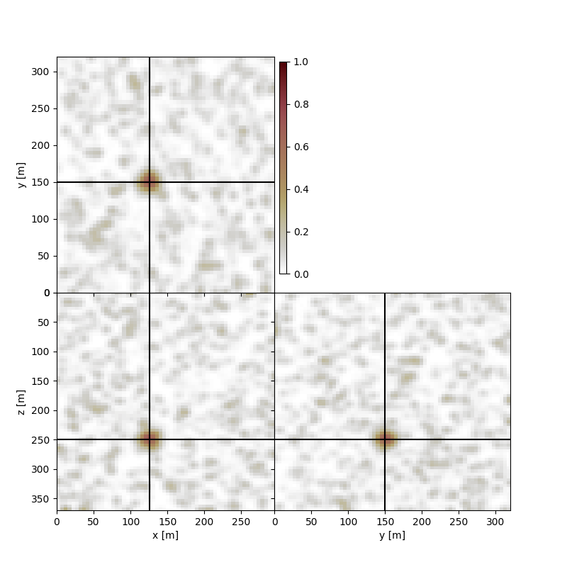
In this example we have a noisy background but the coherent energy, and the image maxima correspond to our source location

noise_inds = np.random.randint(0,nx*ny*nz,size=int(0.05*(nx*ny*nz)))
noise_flat = np.zeros([nx*ny*nz])
noise_flat[noise_inds] = np.random.rand(int(0.05*(nx*ny*nz)))
background_noise = 2*gaussian_filter(noise_flat.reshape([nx,ny,nz]),
                                   sigma=1, radius=2)

microseismic_event = np.zeros_like(background_noise)
microseismic_event[source_location] = 80
microseismic_event = gaussian_filter(microseismic_event, sigma=2, radius=5)
microseismic_image = microseismic_event + background_noise

Perform plotting, here we are going to intersect the volume at the known source location. We also provide the limits for the model space using the xlim, ylim, and zlim parameters.

fig, axs = locimage3d(microseismic_image,
                      x0=int(np.round(source_location[0])),
                      y0=int(np.round(source_location[1])),
                      z0=int(np.round(source_location[2])),
                      xlim=[x[0],x[-1]],
                      ylim=[y[0],y[-1]],
                      zlim=[z[0],z[-1]],
                      clipval=[0,1])
plt.tight_layout()

/home/runner/work/FraCSPy/FraCSPy/fracspy/visualisation/eventimages.py:99: UserWarning: This figure includes Axes that are not compatible with tight_layout, so results might be incorrect.
  fig.tight_layout()
/home/runner/work/FraCSPy/FraCSPy/examples/plot_EventImages.py:58: UserWarning: This figure includes Axes that are not compatible with tight_layout, so results might be incorrect.
  plt.tight_layout()

Noisy Example - Artifact present in image

artifact_location_center = 22, 35, 25  # x,y,z location
artifact_image = np.zeros_like(microseismic_image)
artifact_image[artifact_location_center] = 200
artifact_image = gaussian_filter(artifact_image, sigma=3, radius=4)

microseismic_image_noisy = microseismic_image.copy() + artifact_image

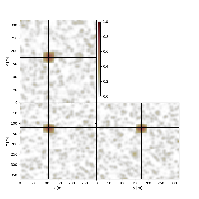
If we perform slicing at the location of the maxima of the image volume we will now be slicing over the artifact location, as opposed to the true source location

max_loc, _ = get_max_locs(microseismic_image_noisy, n_max=5)

fig, axs = locimage3d(microseismic_image_noisy,
                      x0=int(np.round(max_loc[0])),
                      y0=int(np.round(max_loc[1])),
                      z0=int(np.round(max_loc[2])),
                      xlim=[x[0],x[-1]],
                      ylim=[y[0],y[-1]],
                      zlim=[z[0],z[-1]],
                      clipval=[0,1])
plt.tight_layout()

/home/runner/work/FraCSPy/FraCSPy/examples/plot_EventImages.py:87: UserWarning: This figure includes Axes that are not compatible with tight_layout, so results might be incorrect.
  plt.tight_layout()

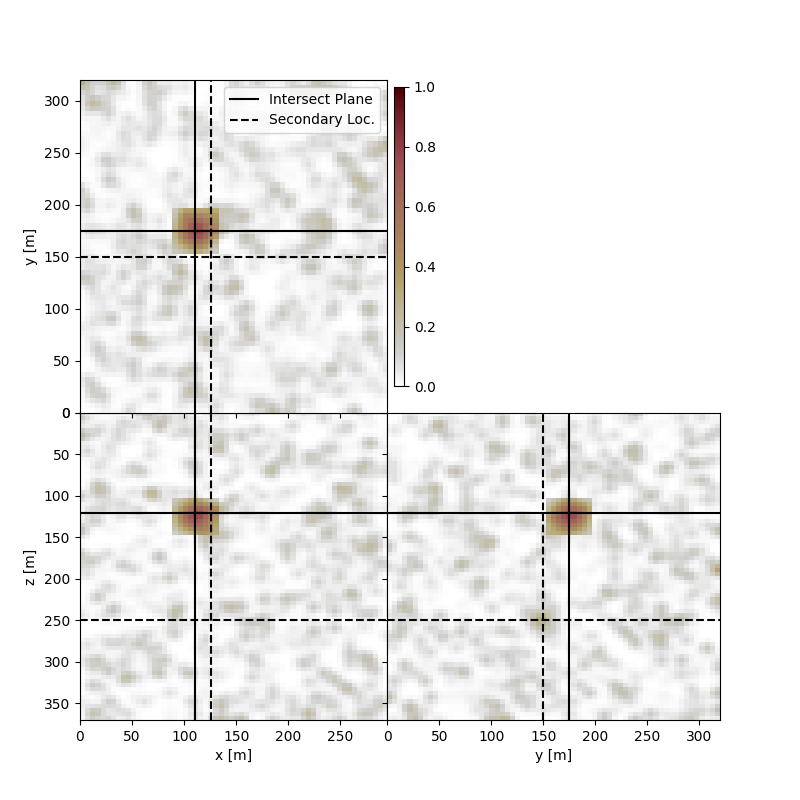
In this instance, it may be preferable to add an additional cross to the plot to highlight where we believe the source location is, in comparison to the maxima for the image volume.

Note, that the source location is not the location for the plane intersection the second cross is merely a projection of the expected location, on top of the intersection.

fig, axs = locimage3d(microseismic_image_noisy,
                      x0=int(np.round(max_loc[0])),
                      y0=int(np.round(max_loc[1])),
                      z0=int(np.round(max_loc[2])),
                      xlim=[x[0],x[-1]],
                      ylim=[y[0],y[-1]],
                      zlim=[z[0],z[-1]],
                      secondcrossloc=source_location,
                      clipval=[0,1])
plt.tight_layout()

/home/runner/work/FraCSPy/FraCSPy/examples/plot_EventImages.py:109: UserWarning: This figure includes Axes that are not compatible with tight_layout, so results might be incorrect.
  plt.tight_layout()