3.1 Amplitude-based Moment Tensor Inversion#

This tutorial illustrates how we can determine the moment tensor of a microseismic source based on the amplitudes of the first P-wave arrival, assuming a known source location.

Starting from the far-field particle velocity expression from a moment tensor source in a homogeneous full space (from eq. 4.29, Aki and Richards):

\[v_i^P = j \omega_P \left( \frac{\gamma_i\gamma_p\gamma_q}{4\pi\rho\alpha^3} \frac{1}{r} \right) M_{pq}\]

where:

\(v\) is the particle velocity measurements (seismic data) at the arrival of the wave, in other words the P-wave peak amplitudes;
\(M\) is the moment tensor;
\(\theta\) describes whether we are utilising the P-wave information;
\(i\) describes the component of the data, aligning with the below p,q definitions;
\(p\) describes the first index of the moment tensor element;
\(q\) describes the second index of the moment tensor element;
\(\omega_P\) is the peak frequency of the given wave;
\(\gamma_{i/p/q}\) is the take-off angle in the i/p/q-th direction (for a ray between the source and receiver);
\(r\) is the distance between source and receiver;
\(\alpha\) is the average velocity (currently we assume a homogeneous velocity);
\(\rho\) is the average density;

If we consider to have access to the vertical particle velocity component of the data (defined here as \(i=1\), the above equation can be expanded out as

\[\begin{split}v_1^P = j \omega_P (\frac{\gamma_1\gamma_1\gamma_1}{4\pi\rho\alpha^3} \frac{1}{r} )M_{1,1} + j \omega_P ( \frac{\gamma_1\gamma_2\gamma_2}{4\pi\rho\alpha^3} \frac{1}{r} )M_{2,2} + j \omega_P ( \frac{\gamma_1\gamma_3\gamma_3}{4\pi\rho\alpha^3} \frac{1}{r} )M_{3,3} + \\ 2*j \omega_P ( \frac{\gamma_1\gamma_1\gamma_2}{4\pi\rho\alpha^3} \frac{1}{r} )M_{1,2} + 2*j \omega_P ( \frac{\gamma_1\gamma_1\gamma_3}{4\pi\rho\alpha^3} \frac{1}{r} )M_{1,3} + 2*j \omega_P ( \frac{\gamma_1\gamma_2\gamma_3}{4\pi\rho\alpha^3} \frac{1}{r} )M_{2,3}\end{split}\]

Here, it is important to recall that the moment tensor matrix is symmetric and can therefore be represented with only 6 elements. This results in the multiplication by two of the off-diagonal elements in the equation above. For more information on the creation of the Greens equations, refer to the source code documentation.

At this point, we can set up a linear problem of the form:

\[\mathbf{v} = \mathbf{G}\mathbf{M}\]

where \(\mathbf{v}\) contains the vertical particle velocity measurements at each receiver, \(\mathbf{M}\) contains the six parameters of the moment tensor fo the source, and \(\mathbf{G}\) is a dense matrix of size \(n_r \times 6\) which contains the scalars linking the different components of the moment tensor to the measurements.

Once the problem is defined, the matrix \(\mathbf{G}\) can be explicitly inverted (or by means of an iterative solver) to obtain our best estimate of the moment tensor parameters.

import os
import numpy as np
import matplotlib.pyplot as plt

import fracspy
from fracspy.visualisation.momenttensor_plots import MTBeachball_comparisonplot
# sphinx_gallery_thumbnail_number = 4

Load model and seismic data#

For this example, we will use a toy example of a small homogenous model with a gridded surface receiver array. The data are modelled using the SOFI3D Finite Difference package.

# Directory containing input data
input_dir = '../data/pyfrac_SOFIModelling'

# Loading the model
abs_bounds = 30
dx = dy = dz = 5
nx = 112
ny = 128
nz = 120

# Modelling parameters
dt = 1e-3  # SOFI3D Time sampling rate
t_shift = 160  # Time shift required to align FD data to zero for Kirchhoff operators
tdur = 500  # Recording duration

# Load model
mod_w_bounds = np.fromfile(os.path.join(input_dir,'inputs',
                                        'models',
                                        'Homogeneous_xyz.vp'),
                           dtype='float32').reshape([nx, ny, nz])

# Load receiver geometry
recs_xzy = np.loadtxt(os.path.join(input_dir,'inputs/griddedarray_xzy_20m.dat')).T
nr = recs_xzy.shape[1]

# Load seismic data
expname = 'MT-90-90-180_Homogeneous_griddedarray'
vz = fracspy.utils.sofiutils.read_seis(
    os.path.join(input_dir, 'outputs',
                 'su', f'{expname}_vy.txt'),
    nr=nr)
vz = vz[:, t_shift: t_shift + tdur]
efd_scaler = np.max(abs(vz))  # Scaler to make data more friendly
vz /= efd_scaler

# Remove absorbing boundaries from both the model and receiver coordinates
mod = mod_w_bounds[abs_bounds:-abs_bounds, abs_bounds:-abs_bounds, :-abs_bounds] # z has free surface
nx, ny, nz = mod.shape
x, y, z = np.arange(nx) * dx, np.arange(ny) * dy, np.arange(nz) * dz
recs = np.array([recs_xzy[0]-(abs_bounds*dx), recs_xzy[2]-(abs_bounds*dx), recs_xzy[1]])

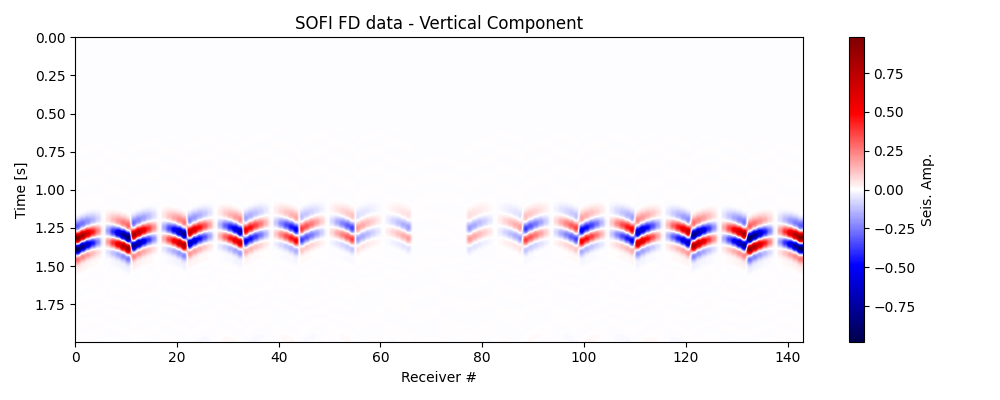
Let’s now double-check that the data has been loaded correctly. Observe the changes in polarity across the traces; this is the information that we utilise to determine the Moment Tensor.

fig, ax = fracspy.visualisation.traceviz.traceimage(vz, climQ=99.99, figsize=(10, 4))
ax.set_title('SOFI FD data - Vertical Component')
plt.tight_layout()

Create modelling operator#

We start by defining the source frequency and location, which we assume to be known ahead of time.

omega_p = 30
sx = nx // 2
sy = ny // 2
sz = 2 * nz // 3
sloc_ind = [sx, sy, sz]

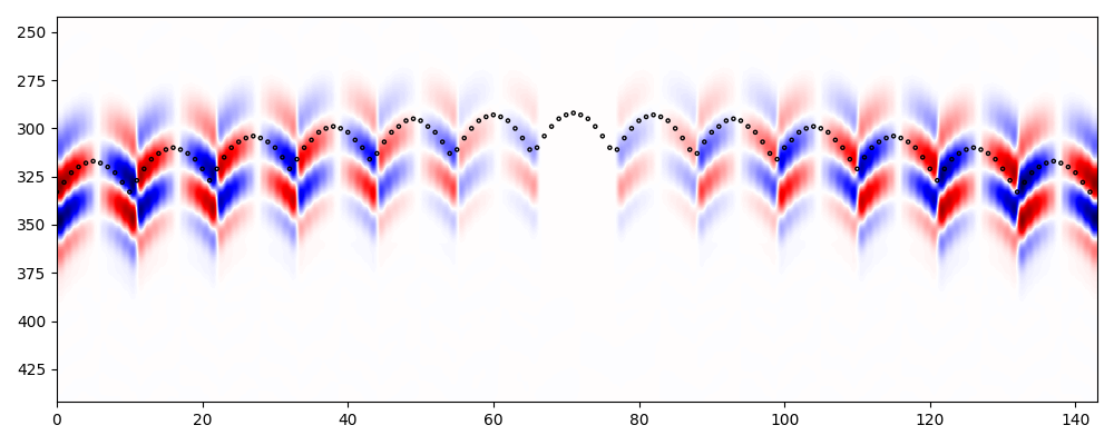
We can now model the traveltimes from the source to each of the receivers and extract the amplitudes at the peak of the P-wave arrival in the data

# Traveltime table
trav = fracspy.modelling.kirchhoff.Kirchhoff._traveltime_table(
        z,
        x,
        y=y,
        recs=recs,
        vel=mod,
        mode='eikonal')
trav = trav.reshape(nx, ny, nz, nr).transpose([3,0,1,2])
source_times = np.round(trav[:, sloc_ind[0],
                        sloc_ind[1], sloc_ind[2]]
                        / dt).astype(int)

# Extract amplitudes at arrival times based on given source location
vz_amps = np.ones(nr)
for i in range(nr):
    vz_amps[i] = vz[i, source_times[i]]

plt.figure(figsize=(10, 4))
plt.imshow(vz[:, np.min(source_times)-50: 150+np.min(source_times)].T,
           aspect='auto', cmap='seismic',
           extent=(0, nr, 150+np.min(source_times), np.min(source_times)-50))
plt.scatter(range(nr), source_times, marker='o', facecolors='none', edgecolors='k', s=5)
plt.tight_layout()

Moment Tensor Inversion#

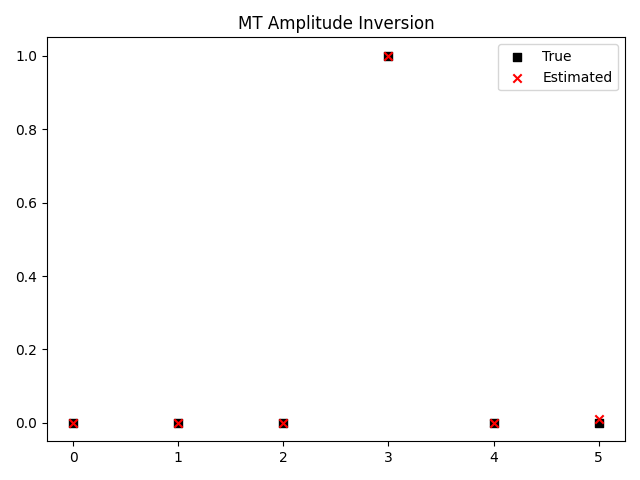
We finally solve our inverse problem to obtain an estimate of the moment tensor

MT = fracspy.mtinversion.MTInversion(x, y, z, recs, mod)
mt_est = MT.apply(vz_amps, sloc_ind, 2, omega_p, kind="ai")
mt_est /= np.max(abs(mt_est))

# Comparison with known MT
mt = np.array([0, 0, 0, 1, 0, 0])
plt.scatter(range(6), mt, c='k', marker='s', label='True')
plt.scatter(range(6), mt_est, c='r', marker='x', label='Estimated')
plt.legend()
plt.title('MT Amplitude Inversion')
plt.tight_layout()

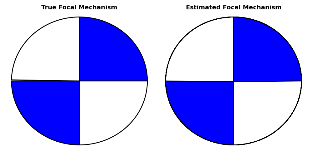
# Beachball comparison plot
MTBeachball_comparisonplot(mt, mt_est)
plt.show()

Total running time of the script: (0 minutes 24.913 seconds)

Gallery generated by Sphinx-Gallery