2.1 Diffraction Stacking: Localisation

This tutorial illustrates how to perform source localisation using diffraction stacking.

We consider here a simple scenario with a homogeneous subsurface model and a point microseismic source with a uniform radiation pattern (explosion-like). We also consider only P-waves for simplicity here, and single-component receivers.

Traveltimes

In a homogeneous medium traveltimes are computed analytically as

\[t(\mathbf{x_r},\mathbf{x_s}) = \frac{d(\mathbf{x_r},\mathbf{x_s})}{v}\]

where \(d(\mathbf{x_r},\mathbf{x_s})\) is the distance between a source at \(\mathbf{x_s}\) and a receiver at \(\mathbf{x_r}\), and \(v\) is medium wave velocity (e.g. P-wave velocity \(v_p\)).

Waveforms

The input data waveforms are computed with the help of PyLops Kirchhoff operator which uses Kirchhoff integral relation with high-frequency Green’s functions.

See more information here: https://pylops.readthedocs.io

Diffraction stacking

The subsurface volume is discretised and each grid node is considered to be a potential source position or a so-called image point. In other words, each image point represents a possible diffraction point from which seismic energy radiates. The term ‘diffraction stacking’ dates back to the works of Claerbout (1971, 1985) and Timoshin (1972). The concept was initially related to seismic migration and imaging of reflectors as a set of diffraction points (in the context of the exploding reflector principle). Here, the diffraction stacking is related to imaging of real excitation sources.

Waveforms from all traces are stacked along the calculated moveouts. In other words, one should apply event moveout (EMO) correction (e.g., Trojanowski and Eisner, 2016) to microseismic data and stack the traces. As the source origin time of a seismic event is unknown, in order to get the image function value \(F(\mathbf{r},t)\), the stacking must be performed for all possible origin times \(t\):

\[F(\mathbf{r},t) = \left|\sum_{R=1}^{N_R} A_R \left(t + T_R(\mathbf{r})\right)\right|,\]

where \(\mathbf{r}\) is a vector that defines a spatial position \((x, y, z)\) of the image point, \(T_R(\mathbf{r})\) is the P-wave traveltime from the image point \(\mathbf{r}\) to a receiver \(R\), \(N_R\) is a number of receivers, and \(A_R\) is the observed waveform at the receiver \(R\) (e.g., Anikiev, 2015).

The term

\[A_R^{EMO}(t,\mathbf{r}) = A_R \left(t + T_R(\mathbf{r})\right)\]

represents the EMO-corrected data.

An absolute value of the stack of the EMO-corrected data is used in order to treat equally positive and negative phases of the stacked amplitudes and let the positive maximum of the resulting 4D image function \(\mathbf{F}_0(\mathbf{r},t)\) work as an indicator of a correct location and origin time of an event (Anikiev et al. 2014).

Another option would be to stack squared values:

\[E(\mathbf{r},t) = \left(\sum_{R=1}^{N_R} A_R^{EMO}(t,\mathbf{r})\right)^2,\]

This simple modification comes from an idea of summation of signal energy rather than the amplitudes (Landa et al. 2006).

However, simple stacking of the absolute or squared values can be further improved, e.g., using a semblance-based approach. The semblance is a coherency or similarity measure and can be understood as the ratio of the total energy (the square of sum of amplitudes) to the energy of individual traces (the sum of squares) (Neidell and Taner, 1971).

For the EMO-corrected data, for image point \(\mathbf{r}\) and a given time step \(t\) the semblance-based image function \(S(\mathbf{r},t)\) can be calculated by:

\[S(\mathbf{r},t) = \frac{\left[\sum_{R=1}^{N_R} A_R^{EMO}(t,\mathbf{r})\right]^2} {N_R \sum_{R=1}^{N_R} \left[A_R^{EMO}(t,\mathbf{r})\right]^2}\]

The main advantage of the semblance-based imaging is its ability to identify and suppress high stack values that result from high noise on only a few receivers, which is a common problem for surface monitoring (Trojanowski and Eisner, 2016). The semblance reaches its maximum value of 1 for identical signals on all traces and the minimum value of 0 for a zero sum of the samples. High stacks resulting from high noise on individual receivers have a low semblance value and in contrast to microseismic events that have consistent amplitude arrivals across the array (provided that EMO correction is done with a suitable velocity model).

In order to suppress the effect of noise even better, it is possible to extend the semblance-based approach by introducing a sliding time window \(W\) over which the energy measures are summed:

\[S_W(\mathbf{r},t,W) = \frac{\sum_{k=it-W}^{it+W}\left[\sum_{R=1}^{N_R} A_R^{EMO}(t,\mathbf{r})\right]^2} {N_R \sum_{k=it-W}^{it+W}\sum_{R=1}^{N_R} \left[A_R^{EMO}(t,\mathbf{r})\right]^2}\]

where \(k\) an index of the time-discretised signal within a sliding time interval consisting of the \(2W + 1\) samples, and \(it\) is the index of time \(t\) (Trojanowski and Eisner, 2016).

Finally, location and origin times of events are determined as the values corresponding to the local maxima of the selected 4-D imaging function.

Assuming that there is only one event in the given time window, its location can be estimated from a 3D volume of the spatial image function obtained by searching for a maximum of \(F(\mathbf{r},t)\) over the time for each spatial point \(\mathbf{r}\):

\[F_s(\mathbf{r}) = F(\mathbf{r},t_{max}(\mathbf{r})),\]

where \(t_{max}\)

\[t_{max}(\mathbf{r}) = \arg\!\max_{t} F(\mathbf{r},t)\]

Alternatively, and average value over time can be computed at each spatial point \(\mathbf{r}\).

The 4-D search is time consuming and if it is necessary to determine only the event location, one can collapse the time dimension by summing the squared image function values over time, e.g.:

\[F_s(\mathbf{r}) = \sum_t F^2(\mathbf{r},t).\]

This idea of summation of the squared image function values here also comes from the path-integral seismic imaging (Landa et al., 2006).

In the end, all the three methods will leave only the spatial dependence, and the estimated event location (hypocenter) \(\mathbf{r}_{est}\) will be associated with the maximum of function \(F_s(\mathbf{r})\):

\[\mathbf{r}_{est} = \arg\!\max_{\mathbf{r}} F_s(\mathbf{r})\]

All the approaches listed above (the various imaging functions as well as the collapsing of the time dimension into a 3D volume) are implemented in fracspy.location.migration.diffstack, and imaging functions with time dimension methods can be used in any combination. However, a combination of summation of the squared values over time with the semblance-based stacking will destroy the scaling of the semblance-based imaging function. To keep the scaling from 0 to 1 while keeping the ability to cover the whole time range, it is advised to use the average over time instead.

Obviously, the absolute-value stacking combined with the summation of the squared values over time will give the same result (up to the scaling coefficient) as the squared-valued stacking combined with the average over time. And if the squared-valued stacking is combined with the summation of the squared values over time it will give a power of 4, which will, of course, provide a more focussed images in a synthetic case, but in case of real data application can be harmful.

Note also that the approach with the maximum value over time is the most universal, because it can provide a reasonable image function for the strongest event even if several events are interfering in one dataset. In this tutorial we have only one microseismic event and we apply the average over time in all cases for comparability. In case of the absolute-value stacking we additionally apply the maximum over time for comparison.

Note that neither of the imaging approaches described here take into account the potential polarity changes of the signal. Therefore, seismograms generated by shear source mechanisms (with positive and negative P-wave and S-wave polarizations) cause these methods to fail to produce high stack values at the true origin time and location because of the destructive interference of the signal (e.g. Anikiev et al., 2014, Trojanowski and Eisner, 2016).

We discuss this issue and introduce diffraction stacking with polarity correction in 2.2 Diffraction Stacking: Localisation With Polarity Correction.

The described localisation methodology allows determination of the source location from the data without picking of arrivals on individual traces. The origin time \(t_{est}\) of the located event can be determined from \(t_{max}\) at the grid point associated with the estimated location \(\mathbf{r}_{est}\) and the corresponding traveltime:

\[\mathbf{t}_{est} = t_{max}(\mathbf{r}_{est}) - \min_{R} T_R(\mathbf{r}_{est}).\]

However, the approach implies that the time window of the processed data contains records only for a single microseismic event, otherwise multiple event signatures will superimpose and image function will become biased.

We discuss this issue as well as joint detection and localisation of multiple events using diffraction stacking in 1.2 Diffraction Stacking: Detection.

References

Anikiev, D. (2015). Joint detection, location and source mechanism determination of microseismic events (Doctoral dissertation). St. Petersburg State University. St. Petersburg. https://disser.spbu.ru/files/phdspsu2015/Anikiev_PhD_web_final.pdf

Anikiev, D., Valenta, J., Staněk, F. & Eisner, L. (2014). Joint location and source mechanism inversion of microseismic events: Benchmarking on seismicity induced by hydraulic fracturing. Geophysical Journal International, 198(1), 249–258. https://doi.org/10.1093/gji/ggu126

Claerbout, J. F. (1971). Toward a unified theory of reflector mapping. Geophysics, 36(3), 467-481. https://doi.org/10.1190/1.1440185

Claerbout, J. (1985). Imaging the earth’s interior. Oxford, England: Blackwell Scientific Publications. https://sepwww.stanford.edu/sep/prof/iei2/

Landa, E., Fomel, S., & Moser, T. (2006). Path‐integral seismic imaging. Geophysical Prospecting, 54(5), 491–503. https://doi.org/10.1111/j.1365-2478.2006.00552.x

Neidell, N. S., & Taner, M. T. (1971). SEMBLANCE AND OTHER COHERENCY MEASURES FOR MULTICHANNEL DATA. Geophysics, 36(3), 482–497. https://doi.org/10.1190/1.1440186

Timoshin Yu. V. (1972). Fundamentals of diffraction conversion of seismic recordings. Moscow: Nedra. [In Russian].

Trojanowski, J., & Eisner, L. (2016). Comparison of migration‐based location and detection methods for microseismic events. Geophysical Prospecting, 65(1), 47–63. https://doi.org/10.1111/1365-2478.12366

Load all necessary packages

import numpy as np
import matplotlib.pyplot as plt

from pylops.utils import dottest
from pylops.utils.wavelets import ricker

# Import modelling utils
from fracspy.modelling.kirchhoff import Kirchhoff
from fracspy.utils.synthutils import add_noise

# Import location utils
from fracspy.location import Location
from fracspy.location.utils import *

# Import visualisation utils
from fracspy.visualisation.traceviz import traceimage
from fracspy.visualisation.eventimages import locimage3d

# Deal with warnings (for a cleaner code)
import warnings
warnings.filterwarnings("ignore", category=FutureWarning)
warnings.filterwarnings("ignore", category=UserWarning)

# Track computation time
from time import time
# sphinx_gallery_thumbnail_number = 13

Setup

Here we setup the parameters of the velocity model, geometry of receivers and microseismic source for forward modelling

Velocity Model

nx, ny, nz = 50, 50, 50
dx, dy, dz = 4, 4, 4
x, y, z = np.arange(nx)*dx, np.arange(ny)*dy, np.arange(nz)*dz

v0 = 1000 # initial velocity
vel = np.ones([nx,ny,nz])*v0

print(f"Velocity model shape: {vel.shape}")

Velocity model shape: (50, 50, 50)

Receivers

dr_xyz = 4*dx

grid_rx_locs = np.arange(dx, (dx*nx)-dx, dr_xyz)
grid_ry_locs = np.arange(dy, (dy*ny)-dy, dr_xyz)

rx, ry, rz = np.meshgrid(grid_rx_locs,
                          grid_ry_locs,
                          dz)
recs = np.vstack((rx.flatten(), ry.flatten(), rz.flatten()))
nr = recs.shape[1]

print(f"Receiver array shape: {recs.shape}")

Receiver array shape: (3, 144)

Microseismic source

isx, isy, isz = [nx//4, ny//2, nz//2]
microseismic = np.zeros((nx, ny, nz))
microseismic[isx, isy, isz] = 1.
sx, sy, sz = isx*dx, isy*dy, isz*dz

Generate synthetic data

start_time = time()
print("Generating synthetic data...")
nt = 81 # number of time steps
dt = 0.004 # time step
f0 = 20 # Central frequency
t = np.arange(nt) * dt # time vector

Generating synthetic data...

Create signal wavelet

wav, wavt, wavc = ricker(t[:41], f0=f0)

Initialise operator

Op = Kirchhoff(z=z,
                x=x,
                y=y,
                t=t,
                recs=recs,
                vel=vel,
                wav=wav,
                wavcenter=wavc,
                mode='eikonal',
                engine='numba')

Check operator with dottest

This test can help to detect errors in the operator implementation.

_ = dottest(Op, verb=True)

Dot test passed, v^H(Opu)=15817.489191526749 - u^H(Op^Hv)=15817.48919152676

Forward modelling

Apply operator to model data

frwddata_1d = Op @ microseismic.flatten().squeeze()
frwddata = frwddata_1d.reshape(nr,nt)

# Contaminate data with white noise
# """""""""""""""""""""""""""""""""

# Fix the seed for reproducibility
seed=1

# Fix SNR levels
snr_wn=1
snr_sn=1/10
snr_rn=1/5

# Fix traces for ringy noise
trind_rn = np.arange(1,nr,11)

# Add white noise of defined SNR
frwddata_wn = add_noise(frwddata,noise_type="white",snr=snr_wn,seed=seed)

# Contaminate data with spiky noise
# """""""""""""""""""""""""""""""""

# Add noise spikes with twice as bigger SNR
frwddata_sn = add_noise(frwddata,noise_type="spiky",snr=snr_sn,seed=seed)

# Contaminate data with ringy noise
# """""""""""""""""""""""""""""""""

# Add ringy noise on some traces
frwddata_rn = add_noise(frwddata,noise_type="ringy",snr=snr_rn,
                        trind=trind_rn,seed=seed)

# Show consumed time
end_time = time()
print(f"Computation time: {end_time - start_time} seconds")

Computation time: 9.758744716644287 seconds

Plot input data

# Plot modelled data
# """"""""""""""""""

fig, ax = traceimage(frwddata, climQ=99.99)
ax.set_title('Noise-free modelled data')
fig = ax.get_figure()
fig.set_size_inches(10, 3)  # set size in inches

Plot modelled data contaminated with white noise

fig, ax = traceimage(frwddata_wn, climQ=99.99)
ax.set_title(f"Modelled data contaminated with white noise of SNR={snr_wn}")
fig = ax.get_figure()
fig.set_size_inches(10, 3)  # set size in inches

Plot modelled data contaminated with spiky noise

fig, ax = traceimage(frwddata_sn, climQ=99.99)
ax.set_title(f"Modelled data contaminated with spiky noise of SNR={snr_sn}")
fig = ax.get_figure()
fig.set_size_inches(10, 3)  # set size in inches

Plot modelled data contaminated with ringy noise

fig, ax = traceimage(frwddata_rn, climQ=99.99)
ax.set_title(f"Modelled data contaminated with ringy noise of SNR={snr_rn}")
fig = ax.get_figure()
fig.set_size_inches(10, 3)  # set size in inches

Plot receiver geometry

fig, ax = plt.subplots(1, 1)
fig.set_size_inches(8, 8)  # set size in inches
ax.set_aspect('equal')
ax.scatter(recs[0],recs[1])
ax.scatter(sx,sy, marker='*')
ax.set_title('Receiver Geometry: map view')
ax.legend(['Receivers', 'Source'],loc='upper right')
ax.set_xlabel('x')
ax.set_ylabel('y')

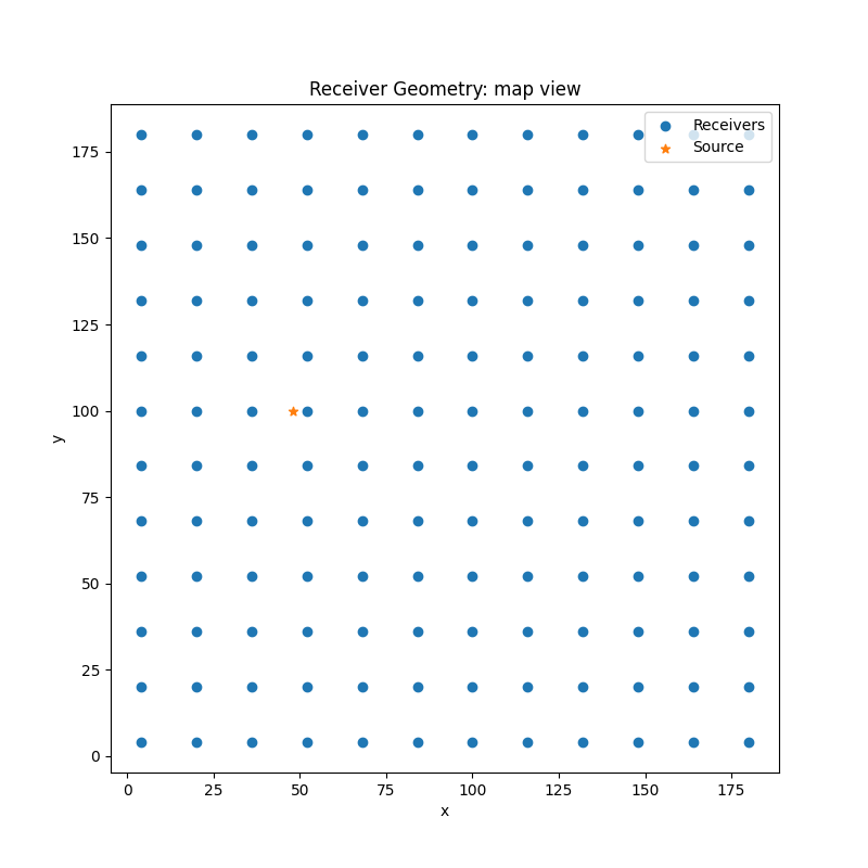
Text(60.347222222222214, 0.5, 'y')

Prepare for location

Define location class using grid vectors

Use the original velocity model grid for location (the grid can be different)

gx = x
gy = y
gz = z

# Set up the location class

L = Location(gx, gy, gz)

Prepare traveltimes

tt = 1 / v0*dist2rec(recs,gx,gy,gz)
print(f"Traveltime array shape: {tt.shape}")

Traveltime array shape: (144, 50, 50, 50)

Apply diffraction stacking to clean data

Here we apply various diffraction stacking algorithms to clean noise-free data, get the image volume and determine location from the maximum of this volume.

Perform absolute-value diffraction stacking

start_time = time()
print("Absolute-value diffraction stacking...")
dstacked_abs, hc_abs = L.apply(frwddata,
                      kind="diffstack",
                      x=gx, y=gy, z=gz,
                      tt=tt, dt=dt, nforhc=10,
                      stack_type="absolute",
                      output_type="mean")
end_time = time()
print(f"Computation time: {end_time - start_time} seconds")

Absolute-value diffraction stacking...
Computation time: 17.846555948257446 seconds

Perform squared-value diffraction stacking

start_time = time()
print("Squared-value diffraction stacking...")
dstacked_sqd, hc_sqd = L.apply(frwddata,
                      kind="diffstack",
                      x=gx, y=gy, z=gz,
                      tt=tt, dt=dt, nforhc=10,
                      stack_type="squared",
                      output_type="mean")
end_time = time()
print(f"Computation time: {end_time - start_time} seconds")

Squared-value diffraction stacking...
Computation time: 17.839326858520508 seconds

Perform semblance-based diffraction stacking without sliding time window

start_time = time()
print("Semblance-based diffraction stacking...")
# Run the stacking using Location class
dstacked_semb, hc_semb = L.apply(frwddata,
                      kind="diffstack",
                      x=gx, y=gy, z=gz,
                      tt=tt, dt=dt, nforhc=10,
                      stack_type="semblance",
                      output_type="mean")
end_time = time()
print(f"Computation time: {end_time - start_time} seconds")

Semblance-based diffraction stacking...
Computation time: 20.4135959148407 seconds

Perform semblance-based diffraction stacking with sliding time window

# Define sliding window as two periods of the signal
swsize = int(2/f0/dt)
print(f"Sliding window size in samples: {swsize}")

start_time = time()
print("Semblance-based diffraction stacking...")
# Run the stacking using Location class
dstacked_semb_swin, hc_semb_swin = L.apply(frwddata,
                      kind="diffstack",
                      x=gx, y=gy, z=gz,
                      tt=tt, dt=dt, nforhc=10,
                      stack_type="semblance", swsize=swsize,
                      output_type="mean")
end_time = time()
print(f"Computation time: {end_time - start_time} seconds")

Sliding window size in samples: 25
Semblance-based diffraction stacking...
Computation time: 24.004881381988525 seconds

Apply diffraction stacking to noise-contaminated data

Here we apply diffraction stacking algorithms to data contaminated with noise.

Perform absolute-value diffraction stacking

start_time = time()
print("Absolute-value diffraction stacking...")
dstacked_abs_wn, hc_abs_wn = L.apply(frwddata_wn,
                            kind="diffstack",
                            x=gx, y=gy, z=gz,
                            tt=tt, dt=dt, nforhc=10,
                            stack_type="absolute",
                            output_type="mean")
dstacked_abs_sn, hc_abs_sn = L.apply(frwddata_sn,
                            kind="diffstack",
                            x=gx, y=gy, z=gz,
                            tt=tt, dt=dt, nforhc=10,
                            stack_type="absolute",
                            output_type="mean")
dstacked_abs_rn, hc_abs_rn = L.apply(frwddata_rn,
                            kind="diffstack",
                            x=gx, y=gy, z=gz,
                            tt=tt, dt=dt, nforhc=10,
                            stack_type="absolute",
                            output_type="mean")
end_time = time()
print(f"Computation time: {end_time - start_time} seconds")

Absolute-value diffraction stacking...
Computation time: 53.57716989517212 seconds

Perform absolute-value diffraction stacking with maximum over time

start_time = time()
print("Absolute-value diffraction stacking...")
dstacked_abs_max_wn, hc_abs_max_wn = L.apply(frwddata_wn,
                            kind="diffstack",
                            x=gx, y=gy, z=gz,
                            tt=tt, dt=dt, nforhc=10,
                            stack_type="absolute",
                            output_type="max")
dstacked_abs_max_sn, hc_abs_max_sn = L.apply(frwddata_sn,
                            kind="diffstack",
                            x=gx, y=gy, z=gz,
                            tt=tt, dt=dt, nforhc=10,
                            stack_type="absolute",
                            output_type="max")
dstacked_abs_max_rn, hc_abs_max_rn = L.apply(frwddata_rn,
                            kind="diffstack",
                            x=gx, y=gy, z=gz,
                            tt=tt, dt=dt, nforhc=10,
                            stack_type="absolute",
                            output_type="max")
end_time = time()
print(f"Computation time: {end_time - start_time} seconds")

Absolute-value diffraction stacking...
Computation time: 51.89684081077576 seconds

Perform squared-value diffraction stacking

start_time = time()
print("Squared-value diffraction stacking...")
dstacked_sqd_wn, hc_sqd_wn = L.apply(frwddata_wn,
                            kind="diffstack",
                            x=gx, y=gy, z=gz,
                            tt=tt, dt=dt, nforhc=10,
                            stack_type="squared",
                            output_type="mean")
dstacked_sqd_sn, hc_sqd_sn = L.apply(frwddata_sn,
                            kind="diffstack",
                            x=gx, y=gy, z=gz,
                            tt=tt, dt=dt, nforhc=10,
                            stack_type="squared",
                            output_type="mean")
dstacked_sqd_rn, hc_sqd_rn = L.apply(frwddata_rn,
                            kind="diffstack",
                            x=gx, y=gy, z=gz,
                            tt=tt, dt=dt, nforhc=10,
                            stack_type="squared",
                            output_type="mean")
end_time = time()
print(f"Computation time: {end_time - start_time} seconds")

Squared-value diffraction stacking...
Computation time: 53.69553828239441 seconds

Perform semblance-based diffraction stacking with sliding time window

# Define sliding window as two periods of the signal
print(f"Sliding window size in samples: {swsize}")
start_time = time()
print("Semblance-based diffraction stacking...")
dstacked_semb_swin_wn, hc_semb_swin_wn = L.apply(frwddata_wn,
                                        kind="diffstack",
                                        x=gx, y=gy, z=gz,
                                        tt=tt, dt=dt, nforhc=10,
                                        stack_type="semblance", swsize=swsize,
                                        output_type="mean")
dstacked_semb_swin_sn, hc_semb_swin_sn = L.apply(frwddata_sn,
                                        kind="diffstack",
                                        x=gx, y=gy, z=gz,
                                        tt=tt, dt=dt, nforhc=10,
                                        stack_type="semblance", swsize=swsize,
                                        output_type="mean")
dstacked_semb_swin_rn, hc_semb_swin_rn = L.apply(frwddata_rn,
                                        kind="diffstack",
                                        x=gx, y=gy, z=gz,
                                        tt=tt, dt=dt, nforhc=10,
                                        stack_type="semblance", swsize=swsize,
                                        output_type="mean")
end_time = time()
print(f"Computation time: {end_time - start_time} seconds")

Sliding window size in samples: 25
Semblance-based diffraction stacking...
Computation time: 72.15548944473267 seconds

Visualisation of results

Here we visualise the slices of the resulting image volume

Plot resulting image volumes from absolute-value diffraction stacking

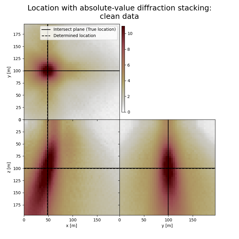
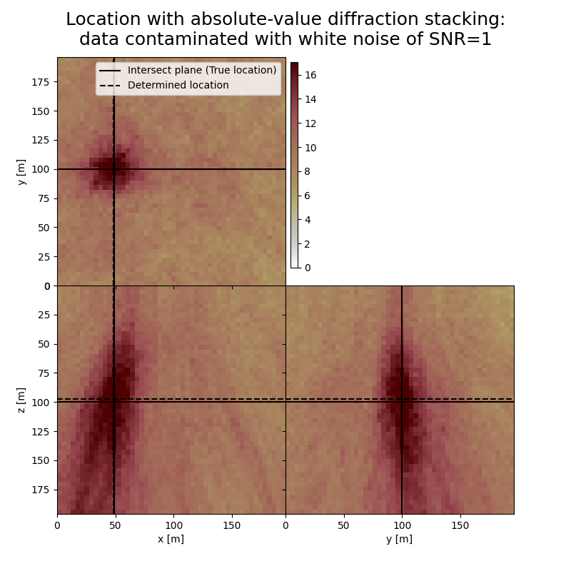
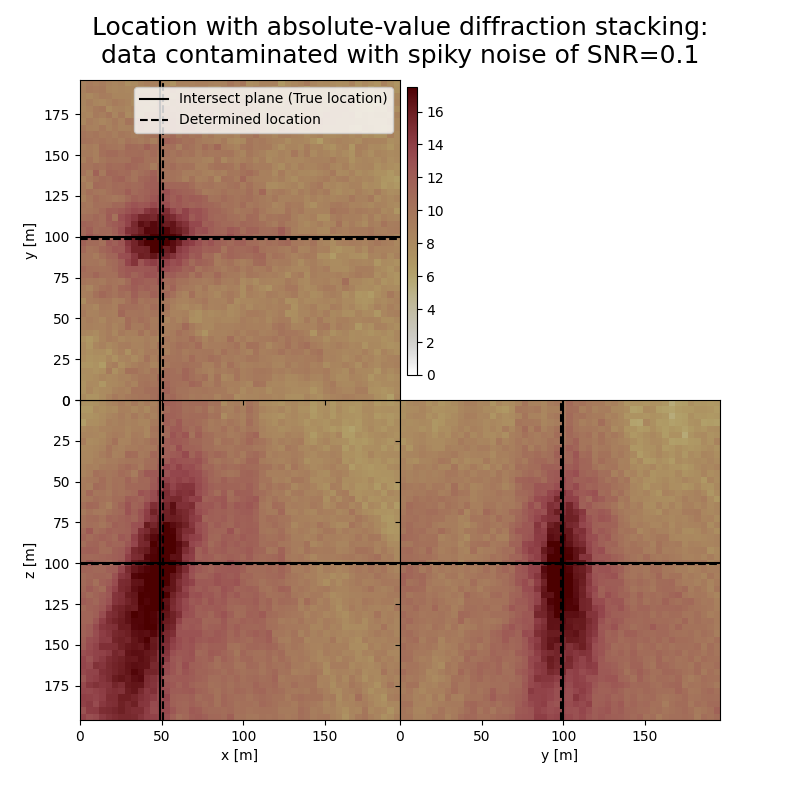
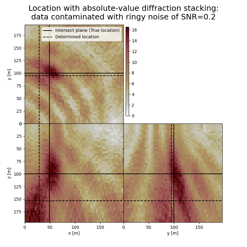
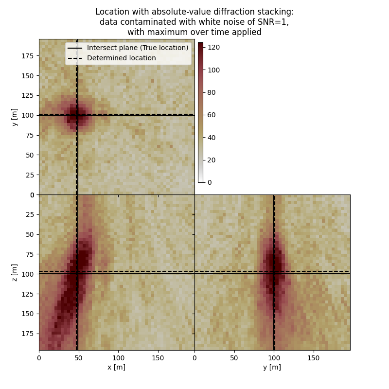
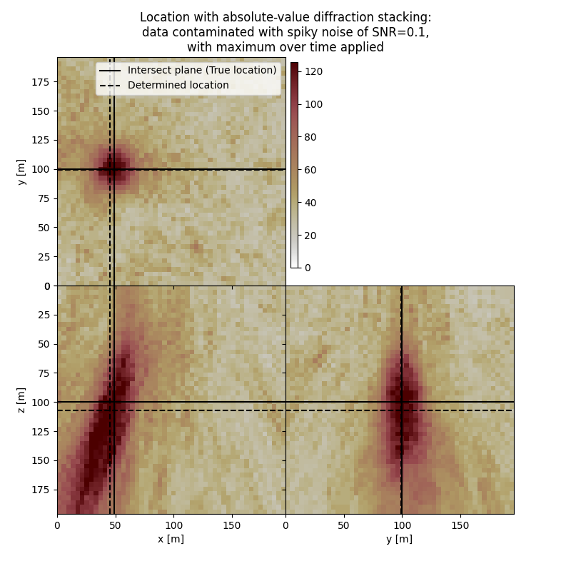
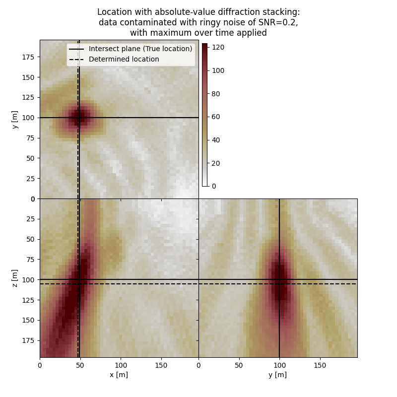
The form and inclination of the location spot reflect the receiver geometry, whereas focusing is related to the selected imaging condition (absolute value). You can see how noise of different kind affects the result. You can also see how changing the output can influence the result.

# Get the spatial limits for plotting
xlim = (min(gx),max(gx))
ylim = (min(gy),max(gy))
zlim = (min(gz),max(gz))

# Define colormap
cmap='cmc.bilbao_r'

# Define legend
crosslegend=('Intersect plane (True location)','Determined location')


# Print true location
print('True event hypocenter:\n[{:.2f} m, {:.2f} m, {:.2f} m]'.format(*[sx, sy, sz]))

# Results of application to clean data:
fig,axs = locimage3d(dstacked_abs,
                     cmap=cmap,
                     title='Location with absolute-value diffraction stacking:\nclean data',
                     x0=isx, y0=isy, z0=isz,
                     secondcrossloc=hc_abs,
                     crosslegend=crosslegend,
                     xlim=xlim,ylim=ylim,zlim=zlim)

print('-------------------------------------------------------')
print('Event hypocenter from absolute-value diffraction stacking for clean data:\n[{:.2f} m, {:.2f} m, {:.2f} m]'.format(*np.multiply(hc_abs,[dx, dy, dz])))
print('Location error:\n[{:.2f} m, {:.2f} m, {:.2f} m]'.format(*get_location_misfit([isx, isy, isz], hc_abs, [dx, dy, dz])))

# Results of application to data contaminated with white noise:
fig,axs = locimage3d(dstacked_abs_wn,
                     cmap=cmap,
                     title=f"Location with absolute-value diffraction stacking:\ndata contaminated with white noise of SNR={snr_wn}",
                     x0=isx, y0=isy, z0=isz,
                     secondcrossloc=hc_abs_wn,
                     crosslegend=crosslegend,
                     xlim=xlim,ylim=ylim,zlim=zlim)
print('-------------------------------------------------------')
print('Event hypocenter from absolute-value diffraction stacking for data contaminated with white noise of SNR={:.1f}:\n[{:.2f} m, {:.2f} m, {:.2f} m]'.format(snr_wn,*np.multiply(hc_abs_wn,[dx, dy, dz])))
print('Location error:\n[{:.2f} m, {:.2f} m, {:.2f} m]'.format(*get_location_misfit([isx, isy, isz], hc_abs_wn, [dx, dy, dz])))

# Results of application to data contaminated with spiky noise:
fig,axs = locimage3d(dstacked_abs_sn,
                     cmap=cmap,
                     title=f"Location with absolute-value diffraction stacking:\ndata contaminated with spiky noise of SNR={snr_sn}",
                     x0=isx, y0=isy, z0=isz,
                     secondcrossloc=hc_abs_sn,
                     crosslegend=crosslegend,
                     xlim=xlim,ylim=ylim,zlim=zlim)
print('-------------------------------------------------------')
print('Event hypocenter from absolute-value diffraction stacking for data contaminated with spiky noise of SNR={:.1f}:\n[{:.2f} m, {:.2f} m, {:.2f} m]'.format(snr_sn,*np.multiply(hc_abs_sn,[dx, dy, dz])))
print('Location error: [{:.2f} m, {:.2f} m, {:.2f} m]'.format(*get_location_misfit([isx, isy, isz], hc_abs_sn, [dx, dy, dz])))

# Results of application to data contaminated with ringy noise:
fig,axs = locimage3d(dstacked_abs_rn,
                     cmap=cmap,
                     title=f"Location with absolute-value diffraction stacking:\ndata contaminated with ringy noise of SNR={snr_rn}",
                     x0=isx, y0=isy, z0=isz,
                     secondcrossloc=hc_abs_rn,
                     crosslegend=crosslegend,
                     xlim=xlim,ylim=ylim,zlim=zlim)
print('-------------------------------------------------------')
print('Event hypocenter from absolute-value diffraction stacking for data contaminated with ringy noise of SNR={:.1f}:\n[{:.2f} m, {:.2f} m, {:.2f} m]'.format(snr_rn,*np.multiply(hc_abs_rn,[dx, dy, dz])))
print('Location error:\n[{:.2f} m, {:.2f} m, {:.2f} m]'.format(*get_location_misfit([isx, isy, isz], hc_abs_rn, [dx, dy, dz])))

# Results of application to data contaminated with white noise with max over time:
fig,axs = locimage3d(dstacked_abs_max_wn,
                     cmap=cmap,
                     x0=isx, y0=isy, z0=isz,
                     secondcrossloc=hc_abs_max_wn,
                     crosslegend=crosslegend,
                     xlim=xlim,ylim=ylim,zlim=zlim)
fig.suptitle(f"Location with absolute-value diffraction stacking:\ndata contaminated with white noise of SNR={snr_wn},\nwith maximum over time applied")
print('-------------------------------------------------------')
print('Event hypocenter from absolute-value diffraction stacking with maximum over time applied for data contaminated with white noise of SNR={:.1f}:\n[{:.2f} m, {:.2f} m, {:.2f} m]'.format(snr_wn,*np.multiply(hc_abs_max_wn,[dx, dy, dz])))
print('Location error:\n[{:.2f} m, {:.2f} m, {:.2f} m]'.format(*get_location_misfit([isx, isy, isz], hc_abs_max_wn, [dx, dy, dz])))

# Results of application to data contaminated with spiky noise with max over time:
fig,axs = locimage3d(dstacked_abs_max_sn,
                     cmap=cmap,
                     x0=isx, y0=isy, z0=isz,
                     secondcrossloc=hc_abs_max_sn,
                     crosslegend=crosslegend,
                     xlim=xlim,ylim=ylim,zlim=zlim)
fig.suptitle(f"Location with absolute-value diffraction stacking:\ndata contaminated with spiky noise of SNR={snr_sn},\nwith maximum over time applied")
print('-------------------------------------------------------')
print('Event hypocenter from absolute-value diffraction stacking with maximum over time applied for data contaminated with spiky noise of SNR={:.1f}:\n[{:.2f} m, {:.2f} m, {:.2f} m]'.format(snr_sn,*np.multiply(hc_abs_max_sn,[dx, dy, dz])))
print('Location error: [{:.2f} m, {:.2f} m, {:.2f} m]'.format(*get_location_misfit([isx, isy, isz], hc_abs_max_sn, [dx, dy, dz])))

# Results of application to data contaminated with ringy noise with max over time:
fig,axs = locimage3d(dstacked_abs_max_rn,
                     cmap=cmap,
                     x0=isx, y0=isy, z0=isz,
                     secondcrossloc=hc_abs_max_rn,
                     crosslegend=crosslegend,
                     xlim=xlim,ylim=ylim,zlim=zlim)
fig.suptitle(f"Location with absolute-value diffraction stacking:\ndata contaminated with ringy noise of SNR={snr_rn},\nwith maximum over time applied")
print('-------------------------------------------------------')
print('Event hypocenter from absolute-value diffraction stacking with maximum over time applied for data contaminated with ringy noise of SNR={:.1f}:\n[{:.2f} m, {:.2f} m, {:.2f} m]'.format(snr_rn,*np.multiply(hc_abs_max_rn,[dx, dy, dz])))
print('Location error:\n[{:.2f} m, {:.2f} m, {:.2f} m]'.format(*get_location_misfit([isx, isy, isz], hc_abs_max_rn, [dx, dy, dz])))

• 
• 
• 
• 
• 
• 
• 

True event hypocenter:
[48.00 m, 100.00 m, 100.00 m]
-------------------------------------------------------
Event hypocenter from absolute-value diffraction stacking for clean data:
[47.60 m, 100.00 m, 100.80 m]
Location error:
[0.40 m, 0.00 m, -0.80 m]
-------------------------------------------------------
Event hypocenter from absolute-value diffraction stacking for data contaminated with white noise of SNR=1.0:
[47.60 m, 100.00 m, 97.20 m]
Location error:
[0.40 m, 0.00 m, 2.80 m]
-------------------------------------------------------
Event hypocenter from absolute-value diffraction stacking for data contaminated with spiky noise of SNR=0.1:
[49.60 m, 98.40 m, 100.80 m]
Location error: [-1.60 m, 1.60 m, -0.80 m]
-------------------------------------------------------
Event hypocenter from absolute-value diffraction stacking for data contaminated with ringy noise of SNR=0.2:
[27.20 m, 94.80 m, 154.00 m]
Location error:
[20.80 m, 5.20 m, -54.00 m]
-------------------------------------------------------
Event hypocenter from absolute-value diffraction stacking with maximum over time applied for data contaminated with white noise of SNR=1.0:
[46.00 m, 101.20 m, 96.80 m]
Location error:
[2.00 m, -1.20 m, 3.20 m]
-------------------------------------------------------
Event hypocenter from absolute-value diffraction stacking with maximum over time applied for data contaminated with spiky noise of SNR=0.1:
[44.00 m, 99.20 m, 107.20 m]
Location error: [4.00 m, 0.80 m, -7.20 m]
-------------------------------------------------------
Event hypocenter from absolute-value diffraction stacking with maximum over time applied for data contaminated with ringy noise of SNR=0.2:
[46.00 m, 100.00 m, 105.20 m]
Location error:
[2.00 m, 0.00 m, -5.20 m]

Plot resulting image volumes from squared-value diffraction stacking

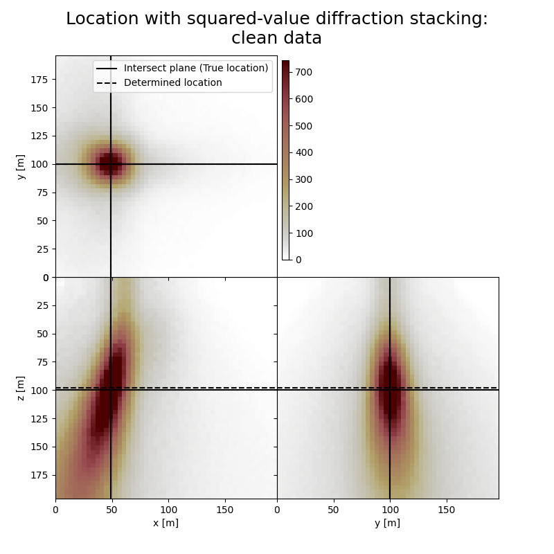
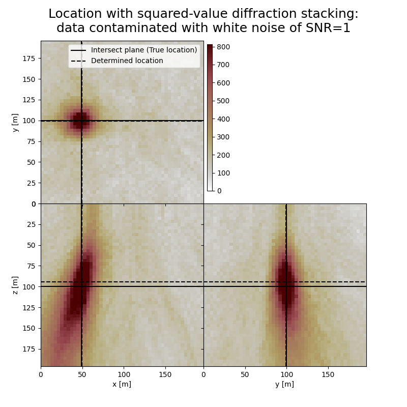
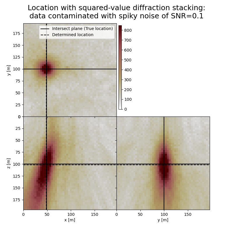
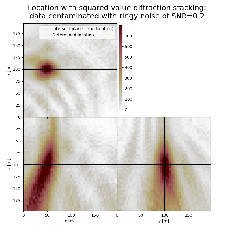
You can see that the focusing is better when using squared values

# Print true location
print('True event hypocenter:\n[{:.2f} m, {:.2f} m, {:.2f} m]'.format(*[sx, sy, sz]))

# Results of application to clean data:
fig,axs = locimage3d(dstacked_sqd,
                     cmap=cmap,
                     title='Location with squared-value diffraction stacking:\nclean data',
                     x0=isx, y0=isy, z0=isz,
                     secondcrossloc=hc_sqd,
                     crosslegend=crosslegend,
                     xlim=xlim,ylim=ylim,zlim=zlim)

print('-------------------------------------------------------')
print('Event hypocenter from squared-value diffraction stacking for clean data:\n[{:.2f} m, {:.2f} m, {:.2f} m]'.format(*np.multiply(hc_sqd,[dx, dy, dz])))
print('Location error:\n[{:.2f} m, {:.2f} m, {:.2f} m]'.format(*get_location_misfit([isx, isy, isz], hc_sqd, [dx, dy, dz])))

# Results of application to data contaminated with white noise:
fig,axs = locimage3d(dstacked_sqd_wn,
                     cmap=cmap,
                     title=f"Location with squared-value diffraction stacking:\ndata contaminated with white noise of SNR={snr_wn}",
                     x0=isx, y0=isy, z0=isz,
                     secondcrossloc=hc_sqd_wn,
                     crosslegend=crosslegend,
                     xlim=xlim,ylim=ylim,zlim=zlim)
print('-------------------------------------------------------')
print('Event hypocenter from squared-value diffraction stacking for data contaminated with white noise of SNR={:.1f}:\n[{:.2f} m, {:.2f} m, {:.2f} m]'.format(snr_wn,*np.multiply(hc_sqd_wn,[dx, dy, dz])))
print('Location error:\n[{:.2f} m, {:.2f} m, {:.2f} m]'.format(*get_location_misfit([isx, isy, isz], hc_sqd_wn, [dx, dy, dz])))

# Results of application to data contaminated with spiky noise:
fig,axs = locimage3d(dstacked_sqd_sn,
                     cmap=cmap,
                     title=f"Location with squared-value diffraction stacking:\ndata contaminated with spiky noise of SNR={snr_sn}",
                     x0=isx, y0=isy, z0=isz,
                     secondcrossloc=hc_sqd_sn,
                     crosslegend=crosslegend,
                     xlim=xlim,ylim=ylim,zlim=zlim)
print('-------------------------------------------------------')
print('Event hypocenter from squared-value diffraction stacking for data contaminated with spiky noise of SNR={:.1f}:\n[{:.2f} m, {:.2f} m, {:.2f} m]'.format(snr_sn,*np.multiply(hc_sqd_sn,[dx, dy, dz])))
print('Location error: [{:.2f} m, {:.2f} m, {:.2f} m]'.format(*get_location_misfit([isx, isy, isz], hc_sqd_sn, [dx, dy, dz])))

# Results of application to data contaminated with ringy noise:
fig,axs = locimage3d(dstacked_sqd_rn,
                     cmap=cmap,
                     title=f"Location with squared-value diffraction stacking:\ndata contaminated with ringy noise of SNR={snr_rn}",
                     x0=isx, y0=isy, z0=isz,
                     secondcrossloc=hc_sqd_rn,
                     crosslegend=crosslegend,
                     xlim=xlim,ylim=ylim,zlim=zlim)
print('-------------------------------------------------------')
print('Event hypocenter from squared-value diffraction stacking for data contaminated with ringy noise of SNR={:.1f}:\n[{:.2f} m, {:.2f} m, {:.2f} m]'.format(snr_rn,*np.multiply(hc_sqd_rn,[dx, dy, dz])))
print('Location error:\n[{:.2f} m, {:.2f} m, {:.2f} m]'.format(*get_location_misfit([isx, isy, isz], hc_sqd_rn, [dx, dy, dz])))

• 
• 
• 
• 

True event hypocenter:
[48.00 m, 100.00 m, 100.00 m]
-------------------------------------------------------
Event hypocenter from squared-value diffraction stacking for clean data:
[48.00 m, 100.00 m, 98.00 m]
Location error:
[0.00 m, 0.00 m, 2.00 m]
-------------------------------------------------------
Event hypocenter from squared-value diffraction stacking for data contaminated with white noise of SNR=1.0:
[48.40 m, 99.20 m, 94.40 m]
Location error:
[-0.40 m, 0.80 m, 5.60 m]
-------------------------------------------------------
Event hypocenter from squared-value diffraction stacking for data contaminated with spiky noise of SNR=0.1:
[47.20 m, 100.00 m, 101.60 m]
Location error: [0.80 m, 0.00 m, -1.60 m]
-------------------------------------------------------
Event hypocenter from squared-value diffraction stacking for data contaminated with ringy noise of SNR=0.2:
[48.80 m, 100.40 m, 104.80 m]
Location error:
[-0.80 m, -0.40 m, -4.80 m]

Plot resulting image volume from semblance-based diffraction stacking

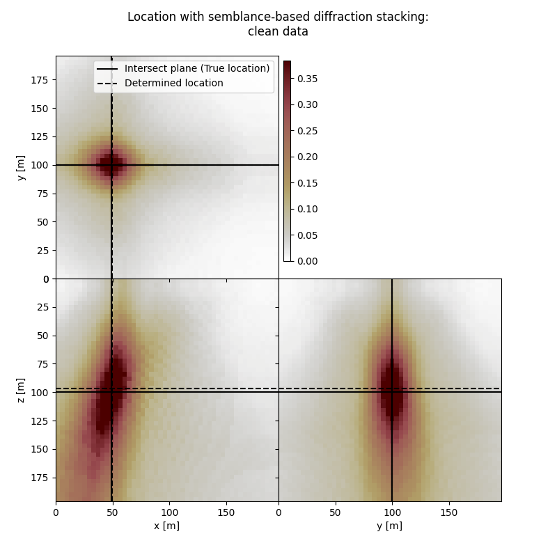
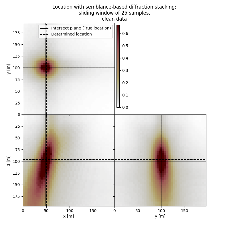
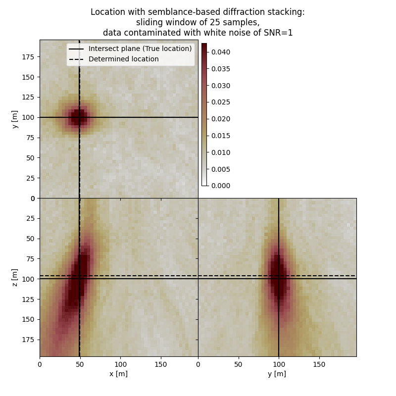
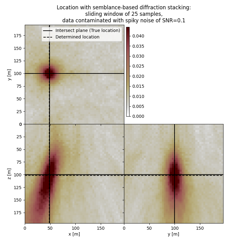
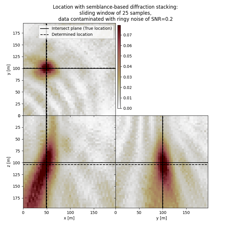
First result show application of semblance-based diffraction stacking without sliding time window. The result has several numerical artifacts. Involving sliding window helps to reduce the artifacts and improve focusing but slightly increases the location error. Semblance-based stacking is generally acting in the presence of noise better than absolute-based stacking.

# Print true location
print('True event hypocenter:\n[{:.2f} m, {:.2f} m, {:.2f} m]'.format(*[sx, sy, sz]))

# Results of application to clean data:
fig,axs = locimage3d(dstacked_semb,
                     cmap=cmap,
                     x0=isx, y0=isy, z0=isz,
                     secondcrossloc=hc_semb,
                     crosslegend=crosslegend,
                     xlim=xlim,ylim=ylim,zlim=zlim)
fig.suptitle("Location with semblance-based diffraction stacking:\nclean data")
print('-------------------------------------------------------')
print('Event hypocenter from semblance-based diffraction stacking for clean data:\n[{:.2f} m, {:.2f} m, {:.2f} m]'.format(*np.multiply(hc_semb,[dx, dy, dz])))
print('Location error:\n[{:.2f} m, {:.2f} m, {:.2f} m]'.format(*get_location_misfit([isx, isy, isz], hc_semb, [dx, dy, dz])))


# Results of application to clean data:
fig,axs = locimage3d(dstacked_semb_swin,
                     cmap=cmap,
                     x0=isx, y0=isy, z0=isz,
                     secondcrossloc=hc_semb_swin,
                     crosslegend=crosslegend,
                     xlim=xlim,ylim=ylim,zlim=zlim)
fig.suptitle(f"Location with semblance-based diffraction stacking:\nsliding window of {swsize} samples,\nclean data")
print('-------------------------------------------------------')
print('Event hypocenter from semblance-based diffraction stacking with sliding window of {:d} samples for clean data:\n[{:.2f} m, {:.2f} m, {:.2f} m]'.format(swsize,*np.multiply(hc_semb_swin,[dx, dy, dz])))
print('Location error:\n[{:.2f} m, {:.2f} m, {:.2f} m]'.format(*get_location_misfit([isx, isy, isz], hc_semb_swin, [dx, dy, dz])))

# Results of application to data contaminated with white noise:
fig,axs = locimage3d(dstacked_semb_swin_wn,
                     cmap=cmap,
                     x0=isx, y0=isy, z0=isz,
                     secondcrossloc=hc_semb_swin_wn,
                     crosslegend=crosslegend,
                     xlim=xlim,ylim=ylim,zlim=zlim)
fig.suptitle(f"Location with semblance-based diffraction stacking:\nsliding window of {swsize} samples,\ndata contaminated with white noise of SNR={snr_wn}")
print('-------------------------------------------------------')
print('Event hypocenter from semblance-based diffraction stacking with sliding window of {:d} samples for data contaminated with white noise of SNR={:.1f}:\n[{:.2f} m, {:.2f} m, {:.2f} m]'.format(swsize,snr_wn,*np.multiply(hc_semb_swin_wn,[dx, dy, dz])))
print('Location error:\n[{:.2f} m, {:.2f} m, {:.2f} m]'.format(*get_location_misfit([isx, isy, isz], hc_semb_swin_wn, [dx, dy, dz])))

# Results of application to data contaminated with spiky noise:
fig,axs = locimage3d(dstacked_semb_swin_sn,
                     cmap=cmap,
                     x0=isx, y0=isy, z0=isz,
                     secondcrossloc=hc_semb_swin_sn,
                     crosslegend=crosslegend,
                     xlim=xlim,ylim=ylim,zlim=zlim)
fig.suptitle(f"Location with semblance-based diffraction stacking:\nsliding window of {swsize} samples,\ndata contaminated with spiky noise of SNR={snr_sn}")
print('-------------------------------------------------------')
print('Event hypocenter from semblance-based diffraction stacking with sliding window of {:d} samples for data contaminated with spiky noise of SNR={:.1f}:\n[{:.2f} m, {:.2f} m, {:.2f} m]'.format(swsize,snr_sn,*np.multiply(hc_semb_swin_sn,[dx, dy, dz])))
print('Location error:\n[{:.2f} m, {:.2f} m, {:.2f} m]'.format(*get_location_misfit([isx, isy, isz], hc_semb_swin_sn, [dx, dy, dz])))

# Results of application to data contaminated with ringy noise:
fig,axs = locimage3d(dstacked_semb_swin_rn,
                     cmap=cmap,
                     x0=isx, y0=isy, z0=isz,
                     secondcrossloc=hc_semb_swin_rn,
                     crosslegend=crosslegend,
                     xlim=xlim,ylim=ylim,zlim=zlim)
fig.suptitle(f"Location with semblance-based diffraction stacking:\nsliding window of {swsize} samples,\ndata contaminated with ringy noise of SNR={snr_rn}")
print('-------------------------------------------------------')
print('Event hypocenter from semblance-based diffraction stacking with sliding window of {:d} samples for data contaminated with ringy noise of SNR={:.1f}:\n[{:.2f} m, {:.2f} m, {:.2f} m]'.format(swsize,snr_rn,*np.multiply(hc_semb_swin_rn,[dx, dy, dz])))
print('Location error:\n[{:.2f} m, {:.2f} m, {:.2f} m]'.format(*get_location_misfit([isx, isy, isz], hc_semb_swin_rn, [dx, dy, dz])))

• 
• 
• 
• 
• 

True event hypocenter:
[48.00 m, 100.00 m, 100.00 m]
-------------------------------------------------------
Event hypocenter from semblance-based diffraction stacking for clean data:
[48.80 m, 100.00 m, 96.80 m]
Location error:
[-0.80 m, 0.00 m, 3.20 m]
-------------------------------------------------------
Event hypocenter from semblance-based diffraction stacking with sliding window of 25 samples for clean data:
[50.00 m, 100.00 m, 96.00 m]
Location error:
[-2.00 m, 0.00 m, 4.00 m]
-------------------------------------------------------
Event hypocenter from semblance-based diffraction stacking with sliding window of 25 samples for data contaminated with white noise of SNR=1.0:
[48.80 m, 100.00 m, 96.00 m]
Location error:
[-0.80 m, 0.00 m, 4.00 m]
-------------------------------------------------------
Event hypocenter from semblance-based diffraction stacking with sliding window of 25 samples for data contaminated with spiky noise of SNR=0.1:
[47.60 m, 99.60 m, 102.00 m]
Location error:
[0.40 m, 0.40 m, -2.00 m]
-------------------------------------------------------
Event hypocenter from semblance-based diffraction stacking with sliding window of 25 samples for data contaminated with ringy noise of SNR=0.2:
[49.20 m, 100.40 m, 104.00 m]
Location error:
[-1.20 m, -0.40 m, -4.00 m]